Key Concepts#
derotation is a modular package for reconstructing rotating image stacks acquired via line scanning microscopes. This page covers the core ideas, flow of information, and how the main modules interact.
See the API documentation for a detailed overview of the package.
How derotation works#
Without derotation, movies acquired with a line scanning microscope are geometrically distorted — each line is captured at a slightly different angle, making it hard to register or interpret the resulting images.
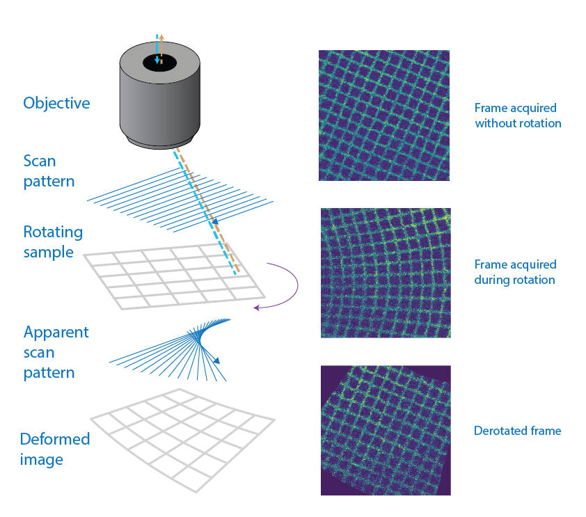
Left: schematic of a line-scanning microscope acquiring an image of a grid. The scanning pattern plus the sample rotation lead fan-like aftefacts. Right: grid that has been imaged while still (top), while rotating (middle) and the derotated image (bottom). The grid is now perfectly aligned.#
If the angle of rotation is recorded, derotation can reconstruct each frame by assigning a rotation angle to each acquired line and rotating it back to its original position. This is what is called derotation-by-line. This process incrementally reconstructs each frame and can optionally include shear deformation correction.
Reconstruction of a frame with derotation. The original frame with deformation is on the left. With subsequent iterations, derotation picks a line, rotates it according to the calculated angle, and adds it to the new derotated frame. The final result is on the right.#
How to use derotation#
There are two main ways to use derotation:
1. Low-level core function#
Use derotation.derotate_by_line.derotate_an_image_array_line_by_line() to derotate an image stack, given:
The original multi-photon movie (expects only one imaging plane)
Rotation angle per line
This is ideal for testing and debugging with synthetic or preprocessed data.
Please refer to the example on how to use the core function for a demonstration of how to use derotation.derotate_by_line.derotate_an_image_array_line_by_line().
2. Full and Incremental Pipeline Classes#
Derotation provides two pre-built pipelines for end-to-end processing:
derotation.analysis.full_derotation_pipeline.FullPipelineAssumes randomized, alternating clockwise and counter-clockwise rotations. It performs:Analog signal parsing
Angle interpolation
Bayesian optimization for center estimation
Line-by-line derotation using
derotation.derotate_by_line.derotate_an_image_array_line_by_line()
derotation.analysis.incremental_derotation_pipeline.IncrementalPipelineAssumes a continuous rotation performed in small increments. Inherits fromFullPipelinebut skips Bayesian optimization. Useful when the center of rotation is known or estimated differently.
Both pipelines accept a configuration dictionary (see the configuration guide) and produce:
A derotated TIFF stack
A CSV file with rotation angles and metadata
Debugging plots
A text file containing the estimated optimal center of rotation
Log files
You can create custom pipelines by subclassing FullPipeline and overriding the relevant methods.
See the usage example for how to instantiate FullPipeline, run it, and inspect its attributes and outputs.
Data Format and Requirements#
These pipelines are designed for a specific experimental setup. They expect analog input signals in a fixed order and may not work out-of-the-box with custom data.
The following inputs are required:
A numpy array of analog signals, with four channels in this order:
Line clock – signals the start of a new line (from ScanImage)
Frame clock – signals the start of a new frame (from ScanImage)
Rotation ON signal – indicates when the motor is rotating
Rotation ticks – used to compute rotation angles (from the step motor)
A CSV file describing speeds and directions of rotation in the following format:
speed,direction
200,-1
200,1
Refer to the configuration guide for more details on specifying file paths and parameters.
Finding the center of rotation#
An accurate center of rotation is crucial for high-quality derotation. Even small errors can produce residual motion in the derotated movie — often visible as circles traced by stationary objects as cells.
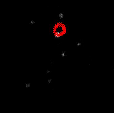
In this picture, you can see as red crosses the centers of one of the cells in the movie across different angles. Since the center is not correctly estimated, the cell appears to move in a circle.#
Derotation offers two approaches for estimating the center:
Bayesian optimization via FullPipeline
This method searches for the correct center of rotation by derotating the whole movie and minimizing a custom metric, computed through the function derotation.analysis.metrics.ptd_of_most_detected_blob(). It requires the average image of the derotated movie at different rotations angles, and from them detects blobs, searches for the most frequent and calculates the Point-to-Point Distance (PTD) for it across blob centers at different rotation angles.
It is robust but computationally expensive.
Ellipse fitting via derotation.analysis.incremental_derotation_pipeline.IncrementalPipeline
This method exploits the fact that incremental datasets rotate very slowly and smoothly. It works by:
Calculate the mean image of the movie at 10 degree rotation intervals
Find the center of the largest blob in each mean image (see
derotation.analysis.blob_detection.BlobDetection)Fitting an ellipse to those centers (this would give you the center of the ellipse, but also the major and minor axes, and the angle of rotation; see the section on out-of-plane rotations for more details on how this information can be used)
The center of the ellipse is assumed to match the true center of rotation. This method fails when the cell stops being visible in certain rotation angles.
Once the center is estimated, it can be fed to the derotation.analysis.full_derotation_pipeline.FullPipeline to derotate the whole movie.
Verifying derotation quality#
Use debugging plots and logs to assess the quality of your reconstruction. These include:
Analog signal overlays
Angle interpolation traces
Center estimation visualizations
Derotated frame samples Debugging plots are by default saved in the
debug_plotsfolder.
You can see some of the debugging plots in the example using real data and the example to find the center of rotation with synthetic data.
Custom plotting hooks#
To monitor what is happening at every step of line-by-line derotation, you can use custom plotting hooks. These are functions that are called at specific points in the pipeline and can be used to visualize intermediate results.
There are two steps in the derotation.derotate_by_line.derotate_an_image_array_line_by_line() function where hooks can be injected:
After adding a new line to the derotated image (
derotation.plotting_hooks.for_derotation.line_addition())After completing a frame (
derotation.plotting_hooks.for_derotation.image_completed())
⚠️ Note: Hooks may slow down processing significantly. Use them for inspection only. You can also inject custom plotting hooks at defined pipeline stages. See the examples page for a demonstration. Note: hooks may significantly slow down processing.
See the plotting hooks example for a demonstration of how to use a custom plotting hook.
Simulated data#
Use the derotation.simulate.line_scanning_microscope.Rotator and derotation.simulate.synthetic_data.SyntheticData classes to generate test data:
derotation.simulate.line_scanning_microscope.Rotator: applies line-by-line rotation to an image stack, simulating a rotating microscope. It can be used to generate challenging synthetic data that include wrong centers of rotation and out of imaging plane rotations.derotation.simulate.synthetic_data.SyntheticData: creates fake cell images, assigns rotation angles, and generates synthetic stacks. This is especially useful for validating both the incremental and full pipelines under known conditions.
This animation shows the synthetic data generated with the Rotator class. As you can see these are two “cells” that rotate around a given center of rotation.#
This is an example of a synthetic dataset with two cells generated with the derotation.simulate.line_scanning_microscope.Rotator class.
Out-of-plane rotations#
A particularly interesting case is when the simulated rotation occurs out of plane, meaning the plane of rotation is not aligned with the imaging plane. In this scenario, the projection of the true 3D rotation onto the 2D imaging plane results in an elliptical trajectory for each cell, rather than a perfect circular path. This trajectory can be captured with the SyntheticData class, or on real data with the IncrementalPipeline class, as the centers of a given cell across different rotation frames. Fitting an ellipse to these points will provide a quantitative estimate of the underlying rotation geometry, including the center of rotation, orientation, and tilt angle of the rotation plane. Orientation refers to the angle of the ellipse in the image plane, which can be calculated from the fitted major and minor axis using the function derotation.analysis.fit_ellipse.derive_angles_from_ellipse_fits(). These parameters can then be used as inputs to the derotation algorithm—specifically by enabling the use_homography option—to perform a more accurate transformation back to the scanning plane. This approach improves derotation performance in cases where the specimen is rotating in 3D space relative to the imaging setup.
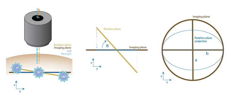
Left: a representation of out of imaging plane rotation paired with the position of a cell at 0deg, 90 deg and 180 deg. Centre: Side view and Right: top view top view of the planes and their relationship with the ellipse that can be fitted to the cell positions.#
You can find different examples on how to use the Rotator and SyntheticData classes in the examples page: